Notes on Convolutional Neural Network

Preliminary knowledge of computer vision is good for readers.
You may also like articles on Image Manipulation and Object Detection.
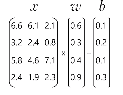
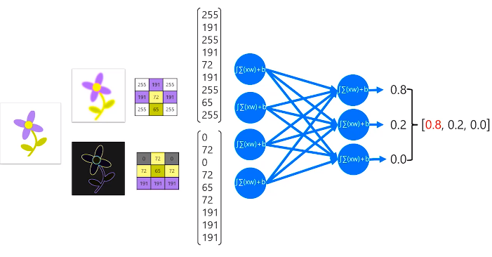
We start with a simple analogy about what is an artificial neuron. It is a math function but a digital one. And it tries to function similar to our brain's neurons. We start off with a simple equation y = f(x, w, b) where y is label output and x input w weight and b bias. At the core, the function has the weighted sum of x inputs multiplied by its corresponding w weight and adds the b bias. The given formula would be Σ(x * w) + b.
More we want to simulate a neuron that fires or not based on whether it reaches a specific threshold or not.
Wrap the weighted sum Σ(x * w) + b) in a function that squashes the overall output value within a range from 0 to 1. This is carried out mostly using the popular Sigmoid function that yields an output in the range between 0-1.
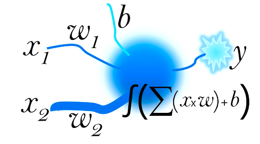
∫(Σ(x * w) + b) is the Activation function which determines whether the artificial neuron fires or not. x1, x2 inputs, w1, w2 weight, b bias and y output.
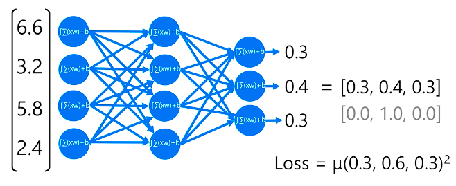
How do neuron functions work to fit in a machine learning model?
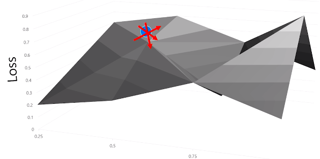
A descending gradient of fn to reduce the loss in multidimensional with varying learning rates.
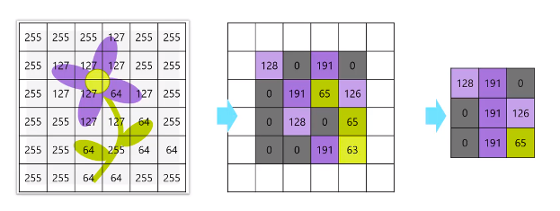
We apply multiple filter kernels each initialized with random weights to the image. Then each of these kernels convolves across the image to produce each one of the feature maps. A ReLU activation function is applied to these feature maps values. ReLU sets negative values to 0 and values greater than 0 as it is.
So after one or more convolutional layers, we use a pooling or downsampling kernel that convolves across the obtained feature map similar to the conv filter layers before. But this downsamples the map by only taking the max values to a smaller feature map to emphasize activated pixels.
Overfitting poses a tough challenge during any convolutional neural network training process. It is the behaviour of a model that learns to classify the training data very well with high accuracy but contrarily fails to generalize the never seen new data on which it hasn’t been trained with lower accuracy.
Building a CNN, we feed training data through network layers in batches, apply a loss function to assess the accuracy of the model and use backpropagation to determine how best to adjust the weights to reduce the loss.
Then similarly we feed validation data except without adjusting weights this time so that we can compare the loss achieved on the data on which the model has never seen or been trained.
Altogether we repeat these two processes multiple times as epochs. And we track each process to collect the statistics for training loss and validation loss as the epochs are complete.
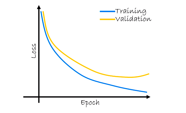
Ideally, both the training loss and validation loss should have a progressive drop that tends to converge. But if the training loss continues to drop and validation loss begins to rise or levels off then the model is clearly overfitting to the training data. It won’t generalize well for new data.
Ways to minimize or mitigate the risk of overfitting during CNN training:
- Randomly drop some of the feature maps generated in the feature extraction layers of the model. It creates some random variability in training data to mitigate overfitting.
- Data augmentation – transforming images in each batch of training data like rotating, flipping etc. This also helps to increase the quantity of the original batches of training data. For eg: a batch of 1000 dog images can be flipped horizontally to generate another set of 1000 dog images.
Combining both ways can help reduce overfitting more efficiently. Data augmentation is always and only performed on training data. Validation data is used as is to check the performance of the model.
Transfer learning
It is easier to learn a new skill if you already have expertise in similar transferable skills.
In a CNN that is trained to extract features from images and identify classes, we can apply a technique like Transfer learning to create a new classifier that builds upon the trained knowledge by the previous model.
Here the pre-trained feature extraction weights that have already been learned to extract edges and corners in the feature extraction layer are not changed. They are retained for use in a new model. However, we replace the fully connected classifier with a new layer that maps the features to classes that we want to identify in input images.
Then train the model by feeding data into it. Only weights and fully connected layers are adjusted. At last, the validation data as usual are used to check the performance of the model.