SARIMA : Seasonal Autoregressive Integrated Moving Average

(p, d, q) (P, D, Q, S)

Time series forecasting model

• predict future values
• extension of non-seasonal ARIMA model
• captures both short term and long term dependencies with data

S - repeating patterns in data

• daily, monthly, yearly regular interval
• key strengths of SARIMA to model seasonality

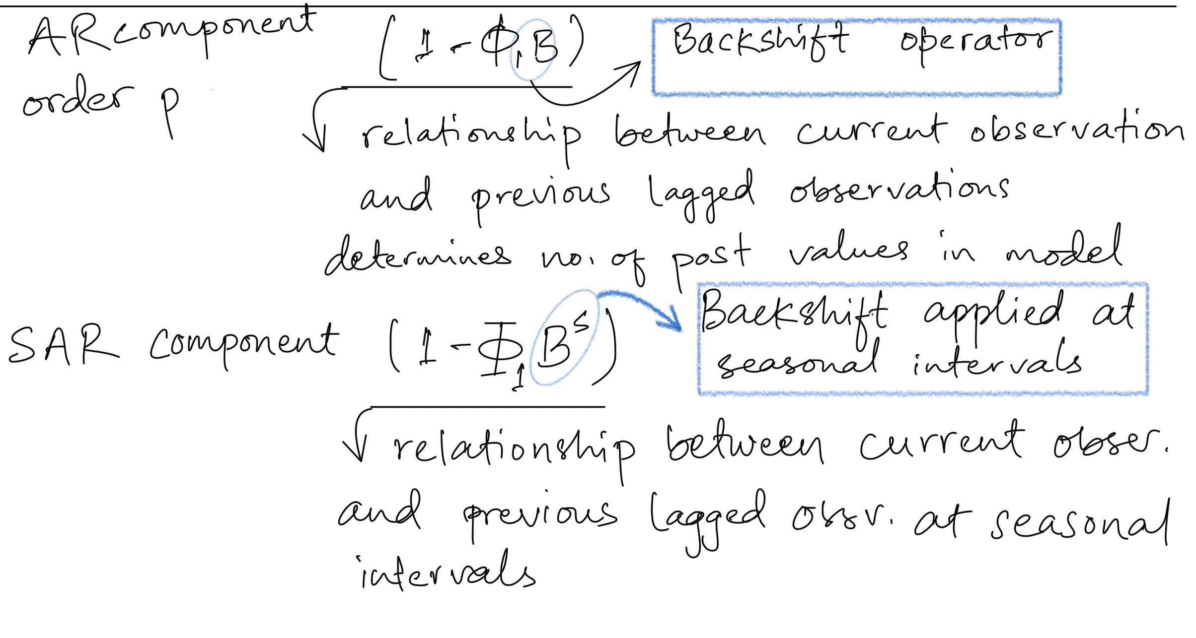
AR (p) - relationship between past and current values

• data autocorrelation
• how correlated data with itself over time

I (d) differencing non stationary data → stationary data

MA (q) dependency between current data point and past prediction errors

captures short term noise in data

Before SARIMA, understand seasonal differencing

subtract time series data by a lag that equals seasonality.
removes seasonal components
makes data stationary
straight forward modeling

• SARIMA assumes time series data is stationary.

Stationarity

• statistical properties of a time series remaining constant over time, such as constant mean, constant variance, and constant autocovariance.
• Dickey-Fuller test is commonly used.
• If p-value less than 0.05, "Stationary"
• otherwise, "Non-Stationary"

SARIMA Notation

SARIMA (p, d, q) (P, D, Q, S)

AR (p) autoregressive component of order P

I (d) integrated component of order d

MA (q) moving average of order q

Seasonal AR (P)
Seasonal MA (Q)
Seasonal I (D)
s : seasonal period

AR component

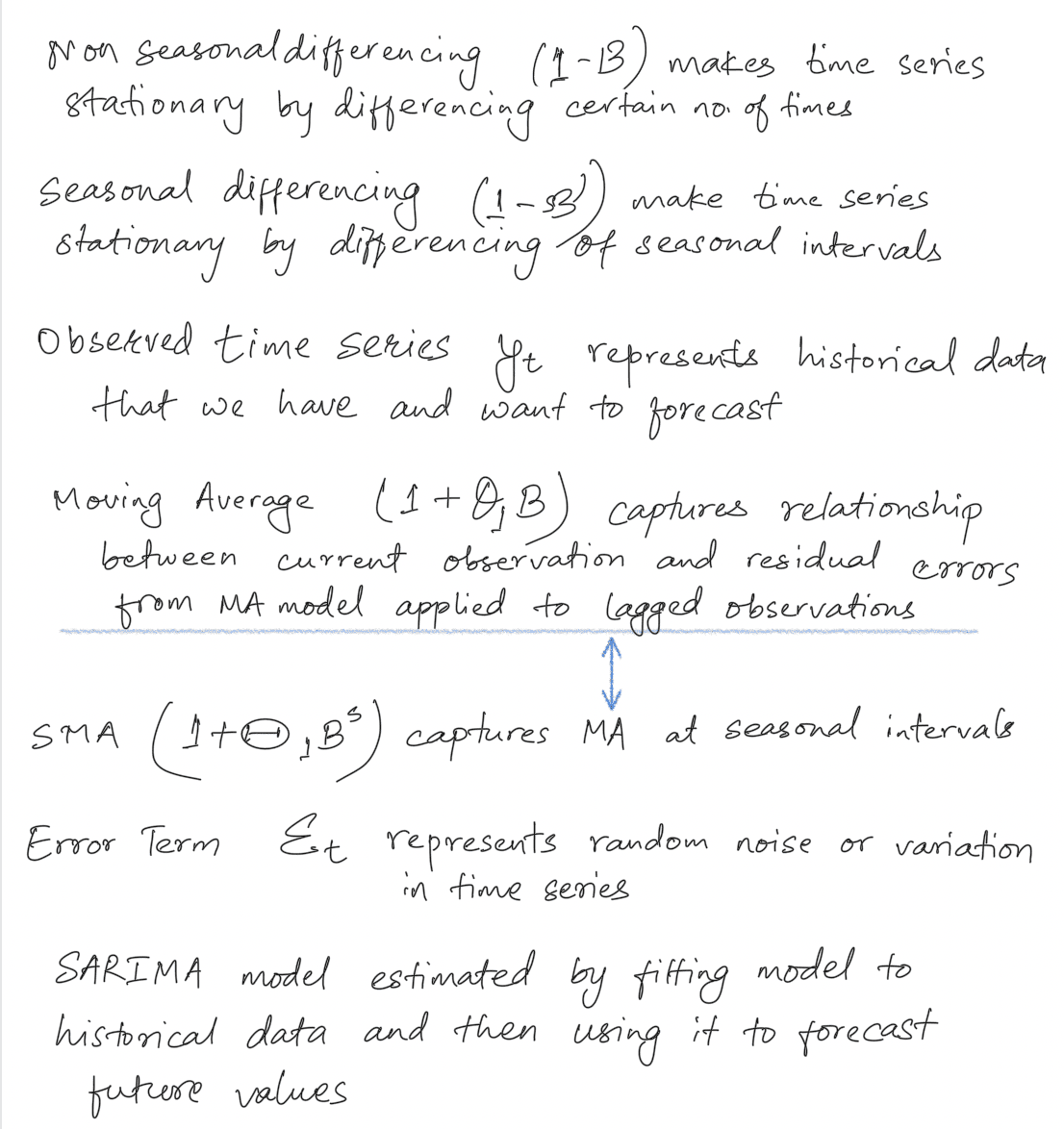
A seasonal difference is the difference between an observation and the previous observation from the same season.

AR - forecast series based on past values called lags

MA - forecast series based on past errors called error lags