Weighted Least Squares - Parameter Estimation

Weighted Least Square is a special case of Generalized Least Square, an extension of Ordinary Least Square

• used in a regression model
• when data points have inconsistent variance of errors
  • i.e. heteroscedasticity
• more weight to good data observations
• less weight to bad or noisy data observations

Using different weights to different data points, WLS tries to minimize the error.

Prior to Weighted Least Square, we need to understand 2 fundamental concepts:

1. variance of errors
2. scedasticity

Variance of Errors - residuals

how much the actual values deviate from the predicted values

• Low variance - predicted values are close to actual values.
  • For eg: model estimated 22 degree weather and it actually feels normal.
• High Variance - predicted values are far from actual values.
  • For eg: model estimated gold price 1 lac but the market price is 2 lacs.

Scedasticity - distribution of error

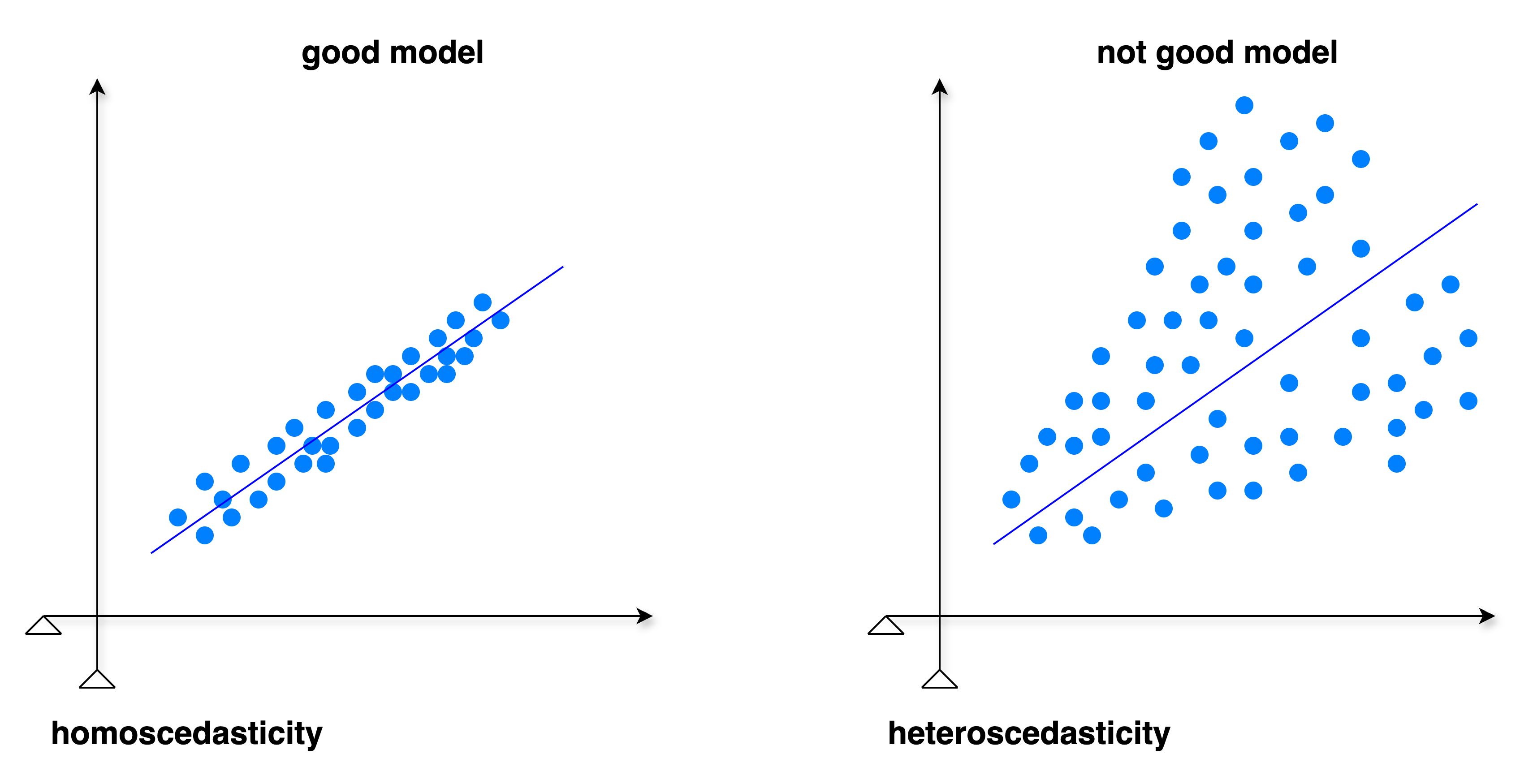
Homoscedasticity - satisfactory model

A “good model” with respect to homoscedasticity means:

1. variance of errors (residuals) are roughly constant: When plotting residuals vs. predicted values, the spread of residuals should not increase or decrease systematically. The plot should look like a horizontal “band” or “cloud” rather than a funnel or cone shape.
2. no patterns in residuals: There should be no obvious trends, curves, or structures in the residuals plot. Patterns indicate that the model is missing some relationship in the data.
3. valid inference: Homoscedasticity ensures that standard errors of coefficients are unbiased, so hypothesis tests (t-tests, F-tests) and confidence intervals are reliable. If heteroscedasticity exists, standard errors may be underestimated or overestimated, leading to invalid inferences.

Heteroscedasticity - unsatisfactory model

A “not good model” with respect to heteroscedasticity means:

• variance of errors (residuals) is not constant across all observations in a regression model.
• this violates a key assumption of Ordinary Least Squares (OLS) regression, which assumes constant variance (homoscedasticity).
• implications for inference:
  • standard errors of coefficients may be biased.
  • confidence intervals and hypothesis tests (t-tests, F-tests) may be unreliable.
  • predictions may have uneven uncertainty, more error where variance is higher.

Formula to find best-fit line in Weighted Least Square

${\beta }_{\mathrm{WLS}}={\left(X^{T}WX\right)}^{-1}{X}^{T}Wy$

• X = input data (independent variables)
• X^T = transpose of X. flips rows and columns of X.
• W = weight
• y = actual values (dependent variables that we want to predict)

$W_i=\frac{1}{{{\sigma }_i}^2}$

W_i = weight assigned to the i-th observation

σ²_i = variance of the error (residual) for the i-th observation

In WLS, Weight is inversely proportional to variance.

Variance is how much data spreads out from the mean.

WLS gives more importance to “trustworthy” data points and less to “noisy” ones.

$\mathrm{Error}={\left(y_{\mathrm{actual}}-y_{\mathrm{predicted}}\right)}^2$ $\mathrm{Weighted\; Error}=W_{i}x{\left(y_{\mathrm{actual}}-y_{\mathrm{predicted}}\right)}^2$ $W_i=weight\; for\; each\; data\; point$ $\mathrm{WLS}=OLS*weights$

---

Weight Least Square in Python

import numpy as np
import statsmodels.api as sm
import matplotlib.pyplot as plt

X = np.array([1, 2, 3, 4, 5])
y = np.array([2.5, 3.5, 5.5, 7.5, 9.0])

# more weight to 3rd data point
weights = np.array([1, 1, 2, 1, 1])

# constant term for intercept
X = sm.add_constant(X)
wls_model = sm.WLS(y, X, weights=weights).fit()

print(wls_model.summary())
y_pred = wls_model.predict(X)

plt.scatter(X[:, 1], y, color='blue', label='Data Points')
plt.plot(X[:, 1], y_pred, color='red', label='WLS Fit')
plt.xlabel("X")
plt.ylabel("y")
plt.legend()
plt.title("Weighted Least Squares (WLS) Fit")
plt.show()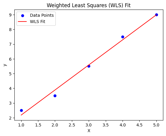

                            WLS Regression Results                            
==============================================================================
Dep. Variable:                      y   R-squared:                       0.989
Model:                            WLS   Adj. R-squared:                  0.986
Method:                 Least Squares   F-statistic:                     281.2
Date:                Wed, 17 Sep 2025   Prob (F-statistic):           0.000462
Time:                        15:04:19   Log-Likelihood:                0.21691
No. Observations:                   5   AIC:                             3.566
Df Residuals:                       3   BIC:                             2.785
Df Model:                           1                                         
Covariance Type:            nonrobust                                         
==============================================================================
                 coef    std err          t      P>|t|      [0.025      0.975]
------------------------------------------------------------------------------
const          0.4833      0.331      1.460      0.240      -0.570       1.537
x1             1.7000      0.101     16.769      0.000       1.377       2.023
==============================================================================
Omnibus:                          nan   Durbin-Watson:                   2.310
Prob(Omnibus):                    nan   Jarque-Bera (JB):                0.371
Skew:                          -0.328   Prob(JB):                        0.831
Kurtosis:                       1.838   Cond. No.                         8.92
==============================================================================

Why use WLS?

• WLS improves accuracy by reducing high variance
• Fixes heteroscedasticity
• Trustworthy data points are weighted. Reliable data are in priority.
• Unreliable data get low weights.

Hence, models can yield more accurate predictions.