Maxout Activation Function
General purpose neuron activation function that outputs maximum value from a set of linear functions in output range (-∞ , ∞)
What is an Activation Function?
An activation (or transfer) function maps a neuron’s weighted inputs plus bias to its output, adding non-linearity so the model can learn complex patterns beyond simple linear ones.
Activation Functions are also known as Transfer Function in the context of Neural Networks.
- Math functions that calculate weighted sum of inputs and adds bias to give non-linearity to output of neuron.
- Decides whether a neuron should be activated (“fired”) or not.
- This helps Neural Network to use important information and suppress not so useful data points.
- Adds non-linearity to Neural Network to tackle complex problems.
- Real-world problems are non-linear. Recognizing cats vs. dogs
- Without activation functions,
f(z) = z, linear regression model, multiple linear layers form up to one big linear equation; useless for non-linear problems.
Maxout Function
piecewise linear function
- General-purpose neuron activation function
- Outputs the maximum value from a set of linear functions.
- Used in hidden layers of deep neural networks as an alternative to ReLU
- Generalizes ReLU and leaky ReLU because it can choose among many.
- Handles vanishing gradients better than sigmoids.
- Requires more parameters, which can increase the model size.
- Good for Dropout regularization (Maxout works very well with it).
- Output range (-∞ , ∞)
Maxout - Mathematical Derivation
- accepts an input tensor x
- reshapes the axis dimension into two dimensions
- takes maximum along the axis dimension
- returns: Output variable. The shape of the output is same as x except that axis dimension is transformed from M * pool_size to M.
Let x ∈ Rd and wi and bi are the weights and biases for the i-th linear function, and k is the number of such functions.
How to apply Maxout?
Assume these inputs, weights, bias and the pool size of 2:
(Shape: 1x3) Input Xi: [3.2, 1.2, 0.5]
(Shape: 3x4) Weight Wi:[0.2 0.4 0.1 -0.5
0.7 -0.3 0.5 0.2
-0.6 0.8 -0.2 0.9]
(Shape: 4) Bias Vector b = [0.1, -0.2, 0.3, 0.0]
Step 1: Input X dot product W weights
Z1 = 3.2⋅0.2 + 1.2⋅0.7 + 0.5⋅(−0.6) = 0.64 + 0.84 − 0.3 = 1.18
Z2 = 3.2⋅0.4 + 1.2⋅(−0.3) + 0.5⋅0.8 = 1.28 − 0.36 + 0.4 = 1.32
Z3 = 3.2⋅0.1 + 1.2⋅0.5 + 0.5⋅(−0.2) = 0.32 + 0.6 − 0.1 = 0.82
Z4 = 3.2⋅(−0.5) + 1.2⋅0.2 + 0.5⋅0.9 = −1.6 + 0.24 + 0.45 = −0.91
Step 2: Add the bias
1.18 + 0.1 = 1.28
1.32 + (−0.2) = 1.12
0.82 + 0.3 = 1.12
−0.91 + 0.0 = −0.91
Before Maxout pooling: [1.28, 1.12, 1.12, −0.91]
Pool size = 2
So, 2 groups of 2 units.
Step 3: Group based on pool size
Group 1: [1.28, 1.12]
Group 2: [1.12, −0.91]
Step 4: Take max value from each
Group 1 output = max(1.28, 1.12)= 1.28
Group 2 output = max(1.12, −0.91)= 1.12
Final Maxout Output: [1.28, 1.12]
Now, let’s try this example in Python Code with NumPy, PyTorch and TensorFlow.
How to implement Maxout Function in Python?
We will write simple code for implementing Softmax activation function in 3 most popular platforms viz. Numpy, PyTorch and TensorFlow.
All code samples are executable in Google Colab easily.
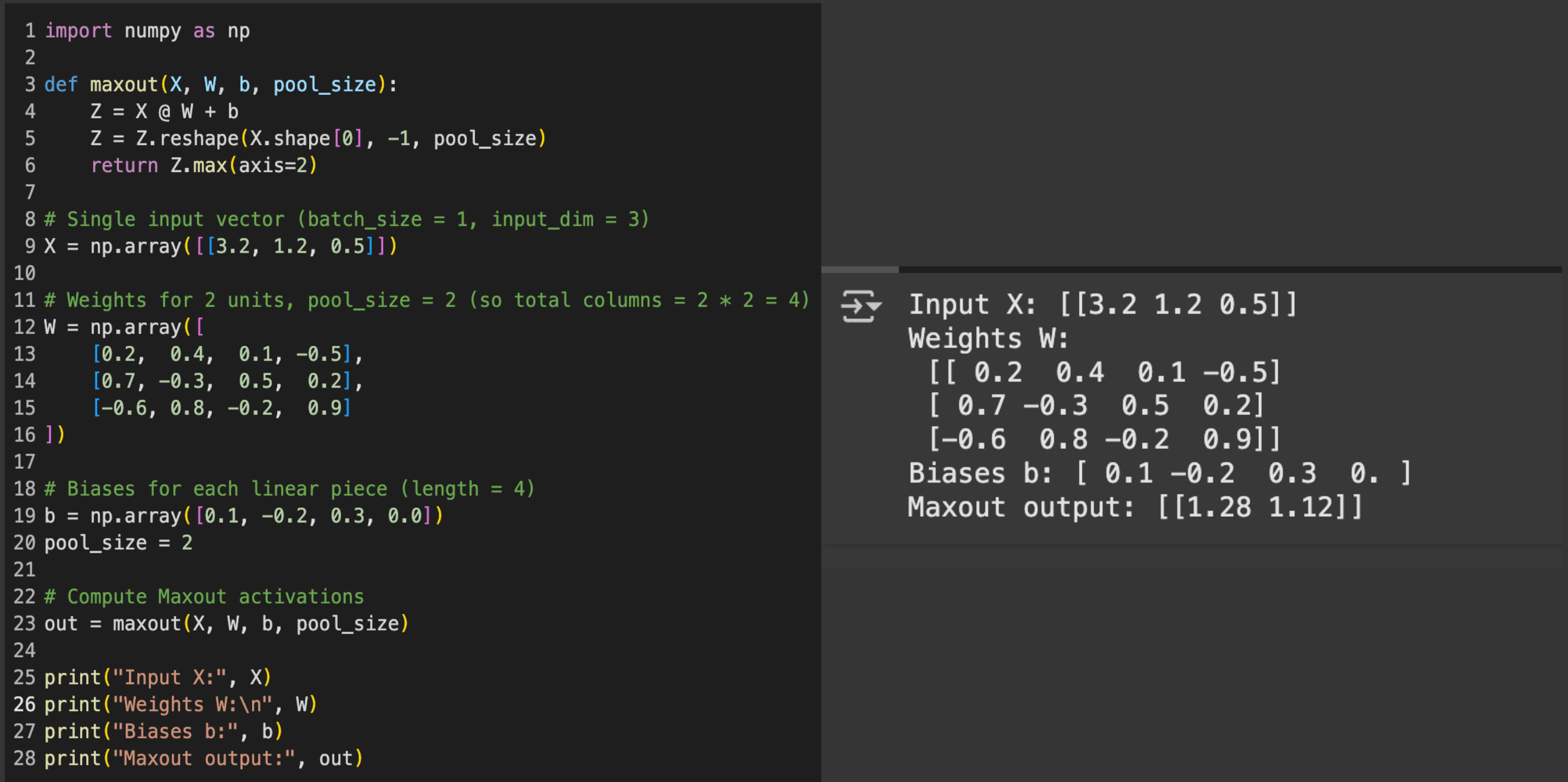
Maxout in Numpy
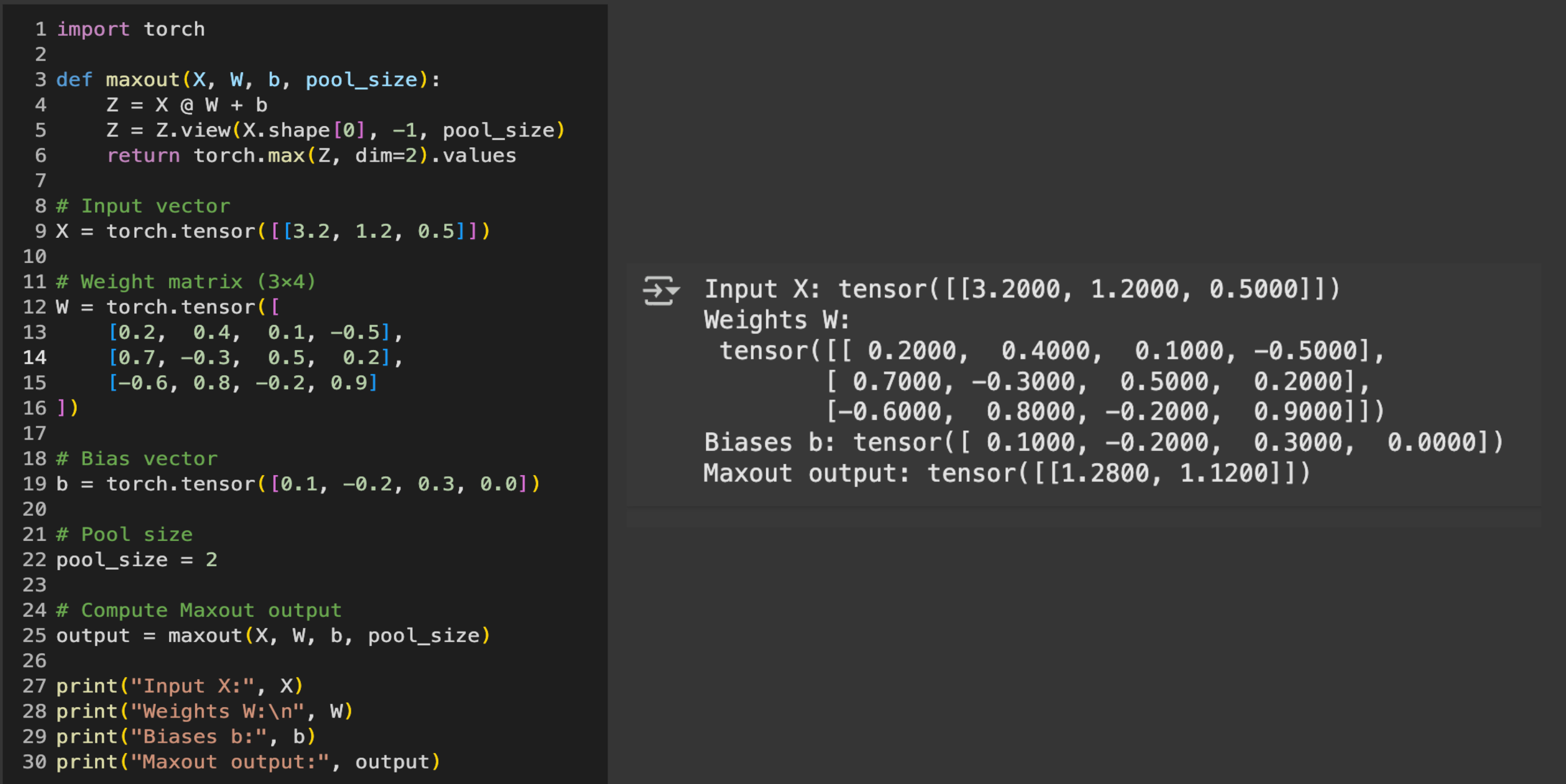
Maxout in PyTorch
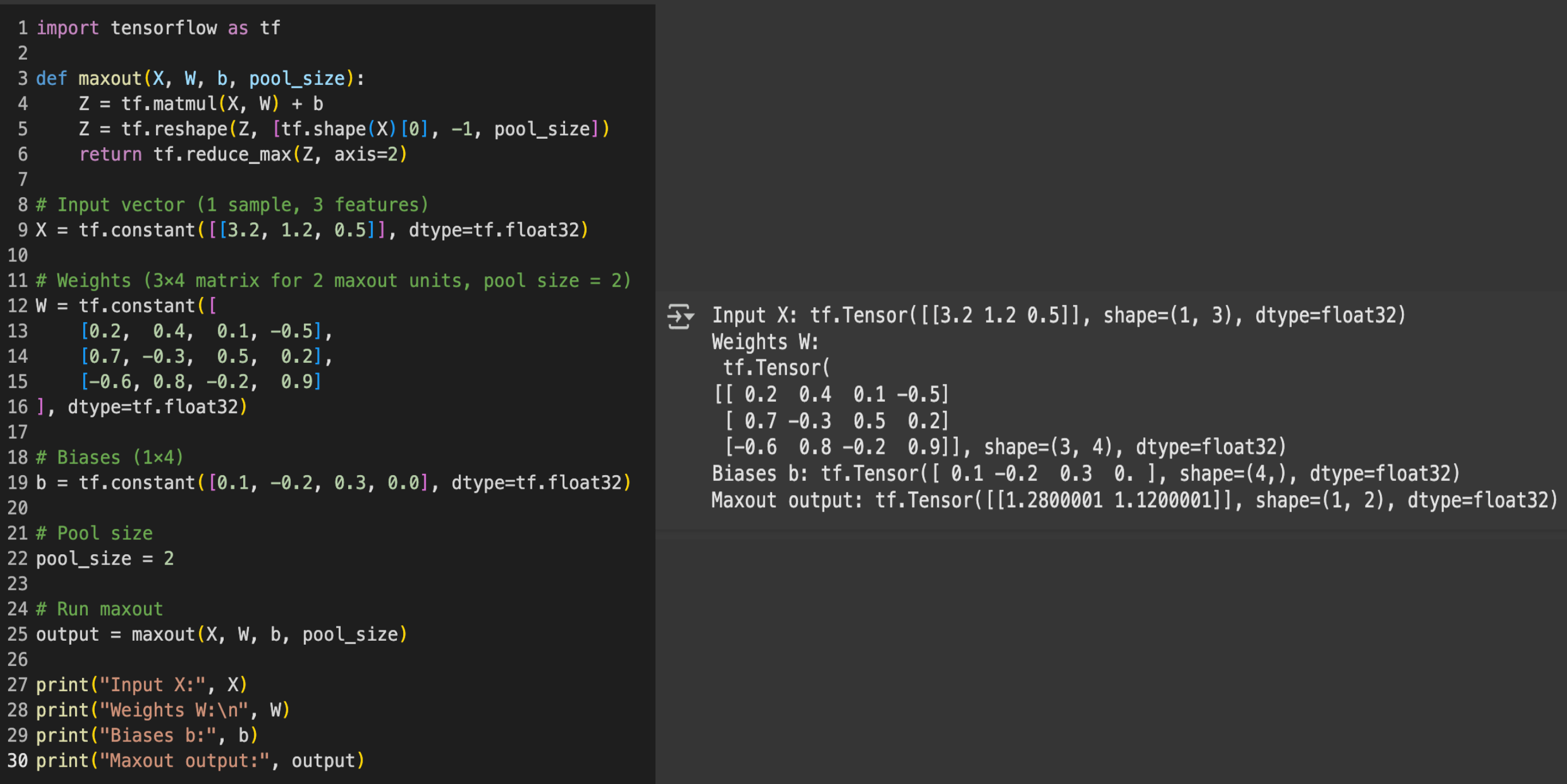
Maxout in TensorFlow
Applications of Maxout
- Object recognition tasks
- Networks dealing with noisy data
- Scenarios needing robustness to vanishing gradients
- Text sentiment analysis
Use case of Maxout
Image Classification Benchmarks
Pairing Maxout with Dropout yields state-of-the-art performance on vision benchmarks such as MNIST, CIFAR-10/100
Text Sentiment Analysis
Doubling convolutional filters (ReLU2x) and using the maxout 3-2 variant achieved the highest sentiment-classification accuracy, outperforming lower-memory activations (LReLU, SeLU, tanh)
Advancements in Maxout Function
Adaptive Piecewise Linear Units
- Unlike Maxout, APLU learns the shape of the activation function during training.
- Offers more expressiveness than Maxout but with fewer parameters.
Mix of Experts (MoE)
- A modular system that picks among multiple expert networks to solve different parts of a task.
- Scalable and adaptive for huge models.
Efficient Approximations
- Efficient approximations are not new functions but rather implementation or architectural strategies to make Maxout more practical
- Reducing computational overhead: Simplifying the Maxout function to require fewer operations.
- Lowering parameter count: Achieving similar performance with fewer learnable parameters.
Comparison between Softmax vs. Maxout
| Topics | Softmax | Maxout |
|---|---|---|
| Concept and Scope | Converts a vector of real-valued scores (logits) into a probability distribution over multiple classes. | Outputs the maximum over multiple linear functions; acts as a general-purpose activation. |
| Mathematical Derivation | softmax(zi) = exp(zi) / Σj exp(zj)Output range: (0, 1) |
f(x) = max(xWi + bi)Output range: (-∞, ∞) |
| Use case scenario | Multi-class classification. Example: classifying handwritten digits in the MNIST dataset. | Useful in speech recognition and text sentiment analysis. |
| Advancements | Adaptive Softmax, Full Softmax, Candidate Sampling, Sparsemax. | Adaptive Piecewise Linear Units (APLU), Maxout Networks, Mixture-of-Experts (MoE). |